Problem 3: Capacity Planning

An Aerospace and Information Systems company was responding to a Request for Proposal from the Internal Revenue Service for an estimated $1 billion modernization plan. A key part of preparing the RFP involved ensuring that the tax returns processing capacity of five IRS regional centers were sufficient at each center to process each tax return within a 17-day time window mandated by Congress. However, overestimating the capacity could contribute to rendering the company's bid less competitive.

Since this daily processing capacity figure (number) was to drive the sizing of the entire architecture for meeting all of the information systems performance specifications, the company wanted to use a systematic approach to determine processing capacity required at each center. A rough-and-ready estimate was acceptable, but the company wanted something more than mere "educated guesses" people were making (and there were many guesses by "eyeballing" various plots of the tax returns arrival data).

Notes

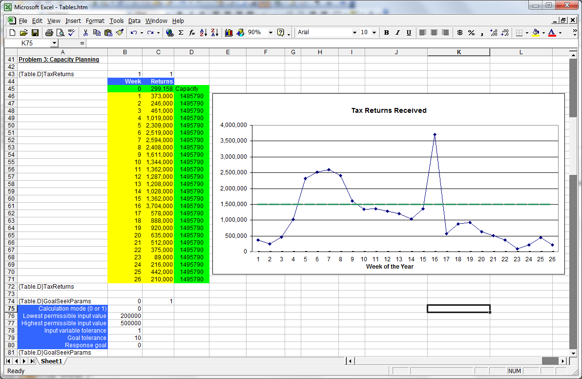
• Excel table (above) shows returns arrival pattern at one of the regional centers during the first 26 weeks of a year

• Returns figure in the table for week zero is not number of returns, but a quick way for communicating to the reader a what-if capacity value to the model. 299,158 and 1,495,790 are daily and 5-day-weekly processing capacities (the answers) that satisfy the goal-seek constraints.

Several assumptions were made to make it possible to develop a quick-and-dirty (yet high confidence) model for determining required processing capacity. They were:

• Returns will be processed on a first-come-first-served basis.

• Weekly returns provided in the table are deterministic.

• Each weekly figure in the table can be spread evenly over the work days of that week.

• All 26 weeks in the table have the same number of work days.

• Service rate is constant per return (in reality, this would be a random variable dependent upon the type of return, the performance levels of data perfecting staff, etc.); every day an equal number of returns will be processed, equal to the capacity of a center, provided, of course, that there are at least that many returns waiting to be processed. 

Formulation of this problem is more easily understood through its ORMSware network diagram and supplemental data files. Click the links further below as desired to open these files in separate windows for reference while reading this document. The mathematical model expressed in the ORMSware diagram below can be viewed by clicking here.

Math model: Original mathematical model of this problem
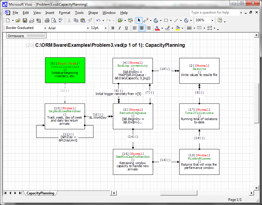
VSD file: Image of Visio network file describing the model
Results: Preview of results of this model.

This model can be implemented in a spreadsheet in a matter of minutes. However, the purpose here is strictly to show how to use the Goalseeking procedure in NMOD's Optimization Module to find minimum cost solution. It will be obvious to the reader that if the bidding company wanted to expand this model to consider variations in arrival patterns and service rates, consequences of expanding work week, introducing overtime, etc., spreadsheet would be a cumbersome environment to continue the modeling.

Following section describes the model:

• Number of returns processed in a day equals either the number of returns waiting to be processed or the daily processing capacity of the center, whichever is less (see expression in display of n[4]Ending inventory).

• Number of returns waiting to be processed at the beginning of any new day is equal to the number of returns left over from previous day plus new arrivals on the new day.

• Leftover returns at the end of the day is equal to the number of returns waiting to be processed at the beginning of the day minus daily processing capacity; if daily capacity is greater than returns waiting at the beginning of the day, leftover at the end of the given day is, obviously, zero.

• Window Capacity is defined as the daily capacity times the length of the window allowed for processing a return. For example, if the daily capacity is 100,000 and the window allowed is 17 days, Window Capacity is 1,700,000.

• Remaining Window Capacity to process new arrivals on a given day is equal to the Window Capacity that will remain after all leftover returns from previous day are processed.

• Number of returns arriving on a day, which cannot be processed within the 17-day window (i.e. number of returns blowing the window constraint), is equal to arrivals for that day minus Remaining Window Capacity. If the Remaining Window Capacity is greater than the arrivals on that day, number of returns blowing the window constraint is zero.

If the Remaining Window capacity on a given day is greater than the arrivals on that day, it may be because the daily service capacity is too large. If the Remaining Window capacity on a given day is less than the arrivals on that day, it is because the daily service capacity is too small. If we calculate the quantity [Daily Violations = Daily Arrivals - Remaining window capacity] for every day, and track the maximum value of Daily Violations over the 26-week horizon, it will tell us whether a daily service capacity is too large or too small.

When this Maximum Daily Violations quantity is negative, it implies that the daily processing capacity is too large. When it is positive, it means that the daily capacity is too small. Therefore, our goal is to find that daily processing capacity which makes the Maximum Daily Violations as close to zero as possible. We can use our descriptive/what-if model to find the minimum capacity solution by using Goalseek from NMOD's Optimization Module to probe the what-if model in a systematic manner.

Execution of this model begins at the green Start node of the network (n[19]Initializations).  n[5]Initializations sets up initial values of several variables, performs certain non-repetitive tasks, and launches the following two cycles in the network:

1. Day and load watcher cycle (n[10]-a[11]-n[10]): This cycle increments the day number each time, round-robins through the days of the week and fetches daily arrivals of returns from the table shown earlier in this document.

2. Inventory tracking and returns processing cycle (n[4]-a[6]-n[3]-a[7]-n[4]): This cycle sets the beginning inventory on a given day equal to the ending inventory from previous day. It also does the day's processing, calculates ending inventory for the day and sends execution threads out for calculating Remaining Window Capacity and tracking daily statistics.

n[5]Initializations: This node is used to do the typical things done in a Start node as you have already seen in previous examples. However, this node also has logic in its SignalTarget property. It sends a signal to a[6]Ending inventory-->>|ReturnsInQueue. This signal is one of the AND triggers that serve to start the tax returns processing cycle described earlier. Whenever a node or arc has content in its SignalTarget property a ^ appears at the end of the top line of that network object's display.

n[10]DayAndLoadWatcher: This node is self-explanatory, but a couple of clarifications may be helpful. strfNxtDayOfWeek is a string function provided by NMOD, which retrieves the next day of the week given current day of the week. It also increments current week number if the next day is a Sunday. WorkDay is a flag used for controlling execution of Inventory tracking and returns processing cycle depending on whether or not a day is a workday.

a[12]DayAndLoadWatcher-->>|ReturnsInQueue: This arc executes only if current day is a workday. Arrival of an entity at n[3]ReturnsInQueue along this arc does not necessarily trigger that node, because this is an AND arc. How things work when an entity reaches n[3]ReturnsInQueue along this arc is further explained under the description of that node.

n[4]Ending inventory: This node calculates returns remaining at the end of each day. In addition to continuing the processing cycle, n[4] also sends execution control to n[2]Results to write daily statistics to a results file.

a[6]Ending inventory-->>|ReturnsInQueue: This arc sets the beginning inventory for next day equal to the ending inventory of current day. It has a duration property of one day, so an entity traveling on it does not reach its termination node n[3]ReturnsInQueue until the next day. Arrival of an entity at along this arc does not necessarily trigger that node, because this is an AND arc. How things work when an entity reaches n[3]ReturnsInQueue along this arc is further explained under the description of that node.

n[3]ReturnsInQueue: While this is a Normal node, it is also a convergence node, because there is at least one AND arc terminating at this node. Convergence nodes fire only when all AND conditions preceding the node are satisfied. In this case, this node will not fire until beginning inventory for a given day is calculated and delivered by a[6]Ending inventory-->>|ReturnsInQueue and number of new arrivals for the day is delivered by n[10]DayAndLoadWatcher along a[12]DayAndLoadWatcher-->>|ReturnsInQueue. It then updates the number of returns waiting in queue to be processed.

a[6]ReturnsInQueue--->|Ending inventory: This arc stops inventory tracking and returns processing cycle as soon as the number of days processed reaches the limit set in n[5]Initializations.

n[15]RemWinCapForNewArr: This node calculates Remaining Window Capacity for processing new arrivals on any given day and sends control to n[13]WindowMisses to calculate number of new arrivals that will miss the required processing window.

n[2]Results: This node for writing daily statistics is also another convergence node in this model. To make sure that this node is fired only once every day and that the daily statistics it writes to the results file is all current, both arcs (a[19] and a[8]) leading into this node are defined to be AND arcs.

Note: It may have appeared to you that some of the nodes in this model have very little content. Looking at the sequence of execution of some of those nodes it may seem that they could easily be combined into one node. This is an important issue. What and how much to incorporate into a node is totally up to the analyst. Factors that are often balanced by the analyst in deciding "how to model it" are clarity, expandability, scalability and execution speed. These are nonfatal judgment factors, since it is possible to change things around fairly easily in NMOD models as the scope of a problem changes.
 

• Click here to view the results file produced by Goalseek. Final results towards the bottom of the file show optimum daily processing capacity.
  
  Viols column in the results file show values of the performance/response variable we chose to measure with Goalseek. Since this column records the highest value (which is what we were interested in) of this response variable, the last value in this column is what Goalseek used to choose the next input value. TotViols column shows how many returns miss acceptable processing window.
  
  
• Click here to view feedback messages to the screen as NMOD's Goalseek searches for the specified goal. If this model were linear, Goalseek would have found the answer with three probes of the model.
  
  
• Click here to view an example of single probe what-if results from this model (using optimal input value found by Goalseek).