UK Retail Chain Transportation Problem

Formulation and solution development Document content writer Target audience Original model and document posting Revisions	Reginald Joules Reginald Joules Quantitative modeling professionals Technical managers Anyone who likes solving problems January 2003 October 2010 May 2012 August 2014


		Reduced image of a small example for explaining the solution technique

Summary

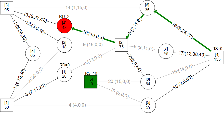
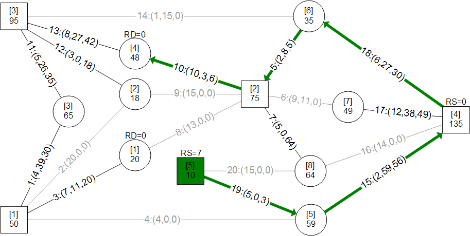
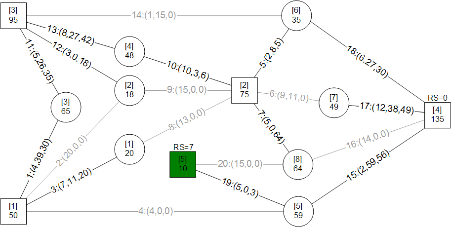
A mass merchandiser in UK wanted a model for minimizing weekly cost of shipping roughly 13 million cases of goods from 9 distribution centers (DCs) to 772 retail stores. I have used an approach here that is easily visualized and implemented through ORMSware to solve this routine business problem typically solved in other ways. This approach thrives on constraints so more can be easily added than the ones presented here. Pease note, however, that Kuhn-Tucker conditions for optimality is not checked in this fast algorithm.

The approach starts with a quick solution (Initial Plan) achieved by sending "probes" simultaneously from every DC to every store it supplies. They reach their targets in ascending order of per-unit shipping costs, allocating all units available at their originating DCs, per the needs of their targets at the moment they reach the targets. If demand at every store can be met this way, a near-optimal answer will have been reached in a split-second.

Chances are, however, that demands at some stores may not be fully met, requiring adjustment of Initial Plan to meet all demands at all stores. When DCs-to-stores flows of units in Initial Plan are changed to meet deficits, total cost increases. Our objective then is to minimize this increase while making the solution feasible (i.e. making sure that all demands at all stores are met without exceeding the original supplies at each DC).

The solution also had to meet another requirement. Each store could only be supplied from 3 DCs closest to it. This restriction meant surplus DCs could not directly supply all deficient stores (else, Initial Plan probes would have achieved a near-optimal solution). The supply restriction was satisfied by systematically increasing and decreasing flows from DCs to stores through minimum cost trades, in just a few iterations, in seconds.

This report is mostly about morphing the infeasible Initial Plan into feasible minimum cost plan by trading flow allocations. A dynamic program (mathematical optimization) is used to find multiple solutions simultaneously during each major iteration and picking minimum cost trade routes. ORMSware makes it easy to visualize and implement this approach and also easy for virtually anyone interested to understand how it works.

Problem

Develop a program for minimizing transportation costs of distributing 13 million cases of goods weekly from 9 distribution centers (DCs) to 772 retail stores of a retail chain. The program should be easily scalable and expandable to meet changing business conditions.

The distribution plan must accommodate the following conditions and requirements:

All DCs are not directly connected to all stores because each store must be supplied by only 3 DCs closest to it
That means that goods cannot be transshipped from a DC to a store through another DC
And also that goods cannot be transshipped from a DC to a store through another store

Background

This is a common linear programming problem with a special structure that is familiar to Operations Research analysts. A software developer contacted me after attempting to solve this problem by explicitly evaluating the costs of all possible combinations of shipping x units from y DCs to z stores. His inquiry and his approach for minimizing total cost are posted here. The retailer's weekly distribution requirements are posted here.

The programmer's routine ran forever without producing answers because total supply of 13 million cases, 9 DCs, 772 stores, and 2316 permissible supply links made evaluating all allowable possibilities indiscriminately through exhaustive enumeration virtually impossible. Within the larger logistics planning picture of a big retail chain, solution to such a transportation problem needs to execute in just seconds.

The speed of the approach presented here is not due to ORMSware or the computer used but due to Operations Research/Management Science. ORMSware simply makes programming the algorithm from scratch easy and highly reliable because the logic is visual, interesting, and easily extendable to impose more constraints as needed.

Results

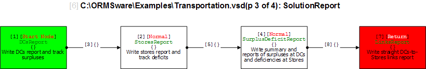
Here is a summary of the answers to the actual problem and links to the results files. Total cost column values reflect UK currency. Explanation of the approach used to solve the problem is provided using a small example further down, below these actual results tables.

Illustration Through Small Example

For easy comprehension of the solution process I will use a small transportation example to explain the solution approach.

Drawing a diagram of the real DC-to-Stores network (781 total nodes and 2316 arcs) on a page would be laborious and meaningless. Fortunately, there is no need to do that since such a network would only be input data which can be expressed in a text file or an Excel worksheet and the algorithm for searching the network for solution can be expressed in ORMSware through just a few logical nodes and arcs.

Data behind the above diagram of the demonstration problem are listed in the table below. It is in the same format in which input data of the actual problem were given to us. Columns of interest are DC_ID, DC_Allowed_Avg_Wk_Cases (weekly supply available at DCs), Store_ID, Total_CPC (per unit shipping cost from a given DC to a given Store), and Store_Avg_Wk_Cases (weekly requirements at stores).

DC_ID	DC_Avg_Wk_Cases	DC_Can_Exceed_By	DC_Allowed_Avg_Wk_Cases	Store_ID	Total_CPC	Store_Avg_Wk_Cases
1	0	0	50	3	4	65
1	0	0	50	2	20	18
1	0	0	50	1	7	20
1	0	0	50	5	4	59
2	0	0	75	6	2	35
2	0	0	75	7	9	49
2	0	0	75	8	5	64
2	0	0	75	1	13	20
2	0	0	75	2	15	18
2	0	0	75	4	10	48
3	0	0	95	3	5	65
3	0	0	95	2	3	18
3	0	0	95	4	8	48
3	0	0	95	6	1	35
4	0	0	135	5	2	59
4	0	0	135	8	14	64
4	0	0	135	7	12	49
4	0	0	135	6	6	35
5	0	0	10	5	5	59
5	0	0	10	8	15	64

Traditional Mathematical Formulation

Let
      x(i,j) = units to be shipped from DC i to Store j, for all j where j is a member of Set T(i) that DC i is allowed to supply, and where i = 1, 2, ..., 9

      c(i,j) = per unit shipping cost from DC i to Store j, for all i and j same as above

      s(i) = number of units available for supply at DC i, where i = 1, 2, ..., 9

      d(j) = number of units required at Store j, where j = 1, 2, ..., 772

Then, we want to minimize

      SUM { c(i,j) * x(i,j) } over all i = 1, 2, ..., 9 and j = 1, 2, ..., 772

Subject to following constraints:

      x(i,j) >= 0 and should be integers

      SUM { x(i,j) } <= s(i) over all j where j is a member of Set T(i)

      SUM { x(i,j) } = d(j) over all i where i is a member of Set U(j) from which Store j is permitted to be supplied

There are many methods for solving this problem. Here we start with a quick and dirty initial solution and then migrate quickly to the optimal solution by implementing a dynamic programming formulation.

ORMSware Approach

ORMSware provides a process-centric object-oriented discrete event simulation approach to solving deterministic and stochastic quantitative modeling problems. Using ORMSware, modelers cause entities known as surrogates, probes, agents, execution threads, etc. to travel through solution networks to produce desired results.

We will say "probes" to refer to surrogates in this discussion, because probe may be an easier conceptual term for visitors who are unfamiliar with ORMSware. Probes carry information and transmit information about various states of the problem as they travel through the model's network.

The transportation problem we are solving here is deterministic and linear. To make model implementation and testing a little easier, we will replace the typical discrete event time dimension with this problem's cost dimension.

For example, in the Initial Plan network shown below probes travel (in the form of signals along a temporal/invisible arc) from node [5] to node [9]. Travel time (duration) of each probe along the temporal arc is replaced by per-unit shipping costs along links connecting each DC to every store it supplies. Probes are launched simultaneously from each DC (represented in node[5]) to all of its target stores (represented in node[9]).

Probes reach node[9] according to their per-unit shipping costs, with the lowest cost probe arriving first and the highest cost probe arriving last.

Initial Plan

As probes reach their target stores Initial Plan starts to take shape according to the following [greedy allocation] logic:

If target store's entire demand has already been fulfilled or if a source DC's supply has already been exhausted by the time this probe arrived at the store, skip to Step 4
Allocate to i-to-j link (DC-to-store link) number of units equal to supply available at DC i, or unfulfilled demand at store j, whichever is less
Subtract units allocated to i-to-j link from supply available at DC i as well as unfulfilled demand at store j
Dispose probe

Notice that the 4 steps listed above ensure that no DC supply constraint is violated and that no store is oversupplied. If all demands are met by the time the last probe is finished at node[9], optimal solution will have been found. If on the other hand not all demands could be met, the solution process enters the MakeItFeasible sub-network.

Node[19] in the network above is a Network node. It represents a sub-network named SolutionReport, which can be found further down on this page. When SolutionReport writes reports of a solution achieved up to any given point, it also tracks DCs with unused/surplus supplies as well as [deficient] stores with unfulfilled demands by entering them into two separate queues for further processing.

If the queue of deficient stores is not empty the solution process enters the Make It Feasible phase represented in yellow node[12] above.

Shown in the diagram below is the Initial Plan for our demo problem. The green nodes are "surplus" DCs with unused supply and red nodes are "deficient" stores with unfulfilled demand. RS and RD values above green and red nodes show remaining unused supplies and unfulfilled demands at those nodes. Arcs/links/connections, also known as decision variables, which are not in the solution "basis" are represented in gray.

Initial Plan

Total Cost = $1573 Unfulfilled demand = 41 units Unfulfilled stores = 2 Surplus DCs = 2

Notice that there are no direct connections between green supply nodes and red demand nodes. This will always be the case, because if they were directly connected surpluses would have been automatically allocated to deficient nodes in the Initial Plan. Therefore, a green node can supply red nodes only by increasing supply to one or more stores it serves, causing a chain reaction that propagates its surpluses to one or more red nodes.

For example, one potential way to get (say) 11 units from green[4] to red[4] is to ship 49 units to store[7], which would make it possible to ship 11 units from DC[2] to red[4] to reduce its deficiency to 10 units.

That trade route is shown in blue in the diagram below. The per-unit cost of doing that trade will be $12 - $9 + $10 = $13, because it will cost $12 to ship a unit from DC[4] to store[7], reduce cost by $9 for not shipping from DC[2] to store[7], and cost $10 to ship from DC[2] to red[4].

For further illumination, let us consider propagating 21 units from green[4] to red[4] via store[6]. Currently DC[2] is not shipping any units to store[6], so there is nothing we can adjust on link 5 from DC[2] to store[6]. The only path to pursue then is link 14 to DC[3] and then link 13 to red[4].

That trade route is shown in pink in the diagram below. The cost of that trade would be $6 - $1 + $8 = $13. So it turns out that costs on the blue trade route and pink trade route are the same.

However, neither of them is the best possible trade at this point, because Green[4]-store[7]-DC[2]-store[6]-DC[3]-store[3]-DC[1]-red[1] (more easily specified with a chain of links 17-6-5-14-11-1-3) offers a better trade at a per-unit cost of $12 - $9 + $2 - $1 + $5 - $4 + $7 = $12. That route is shown in green below. Yes, going to red[4] instead from DC[3] costs the same, too, but I've chosen above route for illustrative purposes.

Those three tradeoff examples illustrate how readjustment of allocations are used to cause red stores in the Initial Plan to be indirectly supplied from green DCs not connected to them. They also promote the need for a method for trading flows in a way that keeps total cost increase to a minimum from iteration to iteration while making sure that already achieved supply and demand constraints are not violated.

Make It Feasible

Since demand at a store cannot be directly fulfilled from other stores or from DCs that are not one of the three DCs permitted to supply it, deficiencies at stores can be rectified only by shuffling (trading) flows allocated in the Initial Plan. We can make sure that total transportation cost increase from iteratively trading off Initial Plan flows to meet all remaining demand requirements is minimized by using a greedy approach once again.

It is a dynamic programming formulation for finding feasible minimum cost trade routes from surplus DCs to deficient stores. The ORMSware network below summarizes this approach. What minimum cost trade routes are and how they are found are explained in detail below the diagram with the aid of a series of snapshots of our small demonstration problem as its solution morphs from infeasible Initial Plan to feasible optimal plan.

The series of diagrams below show how the logic above finds the feasible minimum cost plan. One technical piece of information that may be of interest to some is that the 5 bases below for moving from Initial Plan to the feasible minimum cost solution was found in 3 major iterations (bases 3, 4 and 5 were found in parallel during the 2nd iteration). Discussion of the tradeoff process above can be found after the explanatory diagrams below.

Basis 2

Total Cost = $1705 Cost per unit along minimum cost trade route = $12 Number of units traded = 11
Unfulfilled demand remaining = 30 units Unfulfilled stores = 2 Surplus DCs = 2

Basis 3

Total Cost = $1822 Cost per unit along minimum cost trade route = $13 Number of units traded = 9
Unfulfilled demand remaining = 21 units Unfulfilled stores = 1 Surplus DCs = 2

Basis 4

Total Cost = $2017 Cost per unit along minimum cost trade route = $13 Number of units traded = 15
Unfulfilled demand remaining = 6 units Unfulfilled stores = 1 Surplus DCs = 2

Basis 5

Total Cost = $2059 Cost per unit along minimum cost trade route = $14 Number of units traded = 3
Unfulfilled demand remaining = 3 units Unfulfilled stores = 1 Surplus DCs = 1

Basis 6

Total Cost = $2110 Cost per unit along minimum cost trade route = $17 Number of units traded = 3
Unfulfilled demand remaining = 0 units Unfulfilled stores = 0 Surplus DCs = 1

Final Result of Demo Problem

Total Cost = $2110

Before commencing discussion of the dynamic program for finding optimal trade routes let me show here the sub-network for writing solution reports.

Results of the demo problem are summarized below. Links to results files are listed after the summary.

Major Iteration	Basis	Number of units traded	Cost per unit traded	Total Cost of Plan	Remaining Demand	Number of Deficient Stores	Number of Surplus DCs
Initial Plan	1			$1573	41	2	2
1	2	11	$12	$1705	30	2	2
2	3	9	$13	$1822	21	1	2
2	4	15	$13	$2017	6	1	2
2	5	3	$14	$2059	3	1	1
3	6	3	$17	$2110	0	0	1

File	Description
SupplyFlows1.TXT	Initial Plan results. DCs-to-stores flows and tallies. To-stores-from-DCs flows and tallies.
SupplyFlows2.TXT	Final plan results. DCs-to-stores flows and tallies. To-stores-from-DCs flows and tallies.
Links1.TXT	Initial Plan results. Flows on active links.
Links2.TXT	Final plan results. Flows on active links. Solution difference from Initial Plan.
NMOD.LOG	Execution log. Detailed view of solution process.

Dynamic Program for Finding Optimal Trade Routes

Our objective is to find the lowest cost trade route to make the solution more feasible than it is at any given stage in the solution process. When there are more than one green and one red node every green node is a start point and every red node is a potential end point of the next possible minimum cost trade route. We won't know the best route until one of the probes launched simultaneously from all green nodes reaches a red node.

The search process starts by launching search probes from every green node to all feasible stores. Feasible stores for a DC are all stores that meet the following conditions:

The DC is allowed to supply the store
Current probe has not visited the store before (preventing probe from cycling/getting into an infinite loop)
The store's DC-to-store slack (defined below) is > 0
Cumulative cost (defined below) of reaching the store from green node origin is less than already-found minimum cost trade route to the store

DC-to-Store Slack: It is the difference between a store's original demand and the number of units a DC linked to it is already supplying. For example, in the Initial Plan for our demo problem there was an 11-unit DC-to-store slack from green[4] to store[7] since the store's original demand was 49 units and the DC was supplying only 38.

Cumulative Trading Cost: It is the cost of reaching a node (whether DC or store) along a given trade route from any green node. In our demo example diagram displayed below the Initial Plan, the cumulative trading cost to from DC[4] to store[6] were $6 along the pink trade route and $5 along the green trade route.

Minimum Cumulative Trading Cost: Using the example above, the minimum trading cost to reach store[6] is $5 and the minimum cost trade route to store[6] is the green route from green[4].

Store-to-DC Slack: Somewhat similar to DC-to-store slack, there was a 11 unit slack from store[7] to DC[2] since DC[2] was supplying 11 units to store[7]. Store-to-DC slack is in fact the corresponding DC-to-store flow allocation in the existing solution basis we seek to modify at any given point. We call the flow "slack" because that is the maximum number of units we can push back to the supplying DC to propagate units from green nodes to red nodes.

When search probes are launched from a DC to its feasible stores no attempt is made to gain visibility into what lies beyond those stores. That is because things could change by the time each probe reaches its target/destination store. Even if a probe is calculated to have lower cumulative trading cost to reach a target store than what is in existence at the time it is launched to the store, another probe could reach the target store sooner.

While searching for red nodes, whether a probe is at a green node or any other DC node at any moment, the same rules specified in the 4 bullets above apply for determining the DC's feasible stores. Probes spawned from the arriving probe are then launched to all feasible stores.

When a probe reaches a store its offsprings are launched to all of its feasible DCs. Feasible DCs for a store are all DCs that meet the following conditions:

The store is allowed to be supplied by the DC
Current probe has not visited the DC before
The DC's store-to-DC slack (defined above) is > 0
Cumulative cost (explained above) of reaching the DC from green node origin is less than already-found minimum cost trade route to the DC

Each probe continues to travel this way until it reaches a DC connected to a red store or until it cannot travel further because there are no more feasible targets to pursue. In general, as a probe travels here is what happens as it lands on a DC or store node along the way:

If another probe with lower cumulative trading cost has superseded the arriving probe after it was launched, arriving probe is disposed
If the node a probe lands on has no feasible target nodes, arriving probe is disposed
If a probe survives those two tests it spawns offsprings to travel to current node's feasible target/successor nodes and the arriving probe is disposed

Thus, any probe in play in search of red nodes is always guaranteed to have a trail of minimum cost trade route till the latest node that launched it. When a probe reaches a DC connected to a red store and survives the minimum cost trade route test, it is entered into a queue for creating a matrix of minimum trade route costs. Its offsprings then continue to feasible nodes until there are no more feasible nodes to pursue.

Eventually all probes get disposed, except for the ones entered into the cost matrix described above. When the system becomes quiet all probes in the matrix are launched from their respective DCs to their respective red stores. Simulation clock is reset to zero before the launches and travel duration of each probe is set to cumulative trading cost from its green node origin to its red node destination.

As each probe reaches a red store it is processed the same way probes are handled during Initial Plan phase, except for the following procedure used to calculate how many units can be propagated from the probe's green source node to its red node destination.

Implementation Notes on the Dynamic Program for Finding Optimal Trade Routes

In typical dynamic programming formulation for finding minimum cost paths in a network, costs on all arcs are greater than or equal to zero. Therefore, the probe with minimum cost route from any originating node to any destination node is guaranteed to reach the destination before any other probe. In this problem costs from stores back to their DCs are negative. This situation requires certain additional considerations.

Consider the diagram below you have seen before. The trade route to store[6] at a cost of $5 is the chain of arcs 17-6-5 along the green route. However, since cost/duration on arc 17 is $12 and the duration on arc 18 on the pink route is $6, the probe traveling along arc 18 will reach store[6] first. It will then travel immediately to DC[3] linked to a red store and enter the minimum cost matrix.

To overcome this problem, our algorithm contains logic at each DC and store to let a probe continue even if it arrives at a later time, provided it has a lower cost than the minimum cost route on record at the node. However, the minimum cost matrix has a lowest-cost-out-first queue discipline, and only the first probe of a DC taken out of the queue is sent to the red stores linked to the DC.

Click to go to summaries of all examples